Poisson Lognormal Models • PLNmodels

Description

The Poisson lognormal model and variants¹ can be used for a variety of multivariate problems when count data are at play. This package implements efficient variational algorithms to fit such models, accompanied with a set of functions for visualization and diagnostic. See all the dedicated vignettes for a comprehensive introduction.

PLNmodels covers the following models, all built around the multivariate Poisson-lognormal distribution and sharing a common formula-based interface (covariates, offsets, weights) and a choice of optimization backends (a fast built-in Newton solver, NLOPT, and an experimental torch backend):

PLN²: unpenalized multivariate Poisson regression, with several covariance structures (full, diagonal, spherical, fixed, or a genetic/heritability structure).
PLNPCA³: probabilistic Poisson PCA — a rank-constrained covariance for dimension reduction and visualization.
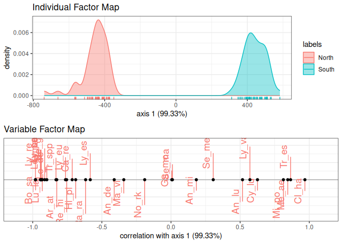
PLNLDA: Poisson lognormal discriminant analysis⁴ for the supervised classification of count data.
PLNnetwork⁵: sparse inverse-covariance (network) inference via a graphical-lasso-like penalty⁶.
PLNmixture: model-based clustering⁷ of count data via a mixture of PLN models.
ZIPLN⁸: a zero-inflated extension of PLN for data with excess zeros, with the same family of covariance structures and an optional sparse (ZIPLNnetwork⁹) variant.

Installation

PLNmodels is available on CRAN. The development version is available on GitHub.

install.packages("PLNmodels")             # last stable version, from CRAN
remotes::install_github("pln-team/PLNmodels")            # development version, from GitHub
remotes::install_github("pln-team/PLNmodels@tag_number")  # a specific tagged release

Illustration

We illustrate the main models on the barents data set¹⁰: the abundance of 30 fish species observed in 89 sites in the Barents sea, along with depth, temperature and geographic coordinates for each site.

library(PLNmodels)

This is package 'PLNmodels' version 1.3.0-9010

data(barents)
## a simple North/South split of the sites, used below to illustrate PLNLDA
barents$zone <- factor(ifelse(barents$Latitude > median(barents$Latitude), "North", "South"))

PLN: fit and inspect the covariance structure

myPLN <- PLN(Abundance ~ Depth + Temperature + offset(log(Offset)), data = barents)

 Initialization...
 Adjusting a full covariance PLN model with nlopt optimizer
 Post-treatments...
 DONE!

myPLN

A multivariate Poisson Lognormal fit with full covariance model.
==================================================================
 nb_param    loglik       BIC       AIC      ICL
      555 -4412.201 -5657.797 -4967.201 -8203.81
==================================================================
* Useful fields
    $model_par, $latent, $latent_pos, $var_par, $optim_par
    $loglik, $BIC, $ICL, $loglik_vec, $nb_param, $criteria
* Useful S3 methods
    print(), coef(), sigma(), vcov(), fitted()
    predict(), predict_cond(), standard_error()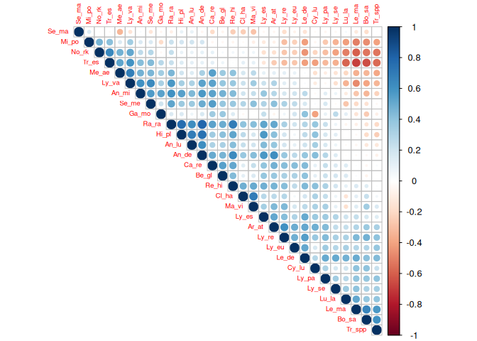

corrplot::corrplot(cov2cor(sigma(myPLN)), order = "AOE", type = "upper", tl.cex = 0.6)

PLNLDA: discriminant analysis

myLDA <- PLNLDA(Abundance ~ offset(log(Offset)), grouping = zone, data = barents)

 Performing discriminant Analysis...
 DONE!

plot(myLDA)

PLNPCA: dimension reduction

myPCAs <- PLNPCA(Abundance ~ Depth + Temperature + offset(log(Offset)), data = barents, ranks = 1:5)

 Initialization...

 Adjusting 5 PLN models for PCA analysis.
     Rank approximation = 1 
     Rank approximation = 2 
     Rank approximation = 3 
     Rank approximation = 4 
     Rank approximation = 5 
 Post-treatments
 DONE!

myPCA  <- getBestModel(myPCAs)
factoextra::fviz_pca_biplot(
  myPCA, select.var = list(contrib = 10), col.ind = barents$Temperature,
  title = "Biplot (10 most contributing species, sites colored by temperature)"
) + ggplot2::labs(col = "Temperature") + ggplot2::scale_color_viridis_c()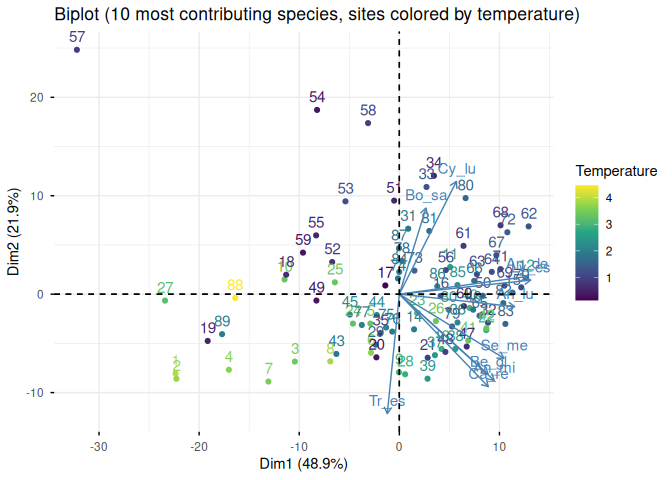

PLNnetwork: sparse network inference

myNets <- PLNnetwork(Abundance ~ Depth + Temperature + offset(log(Offset)), data = barents)

 Initialization...
 Adjusting 30 PLN with sparse inverse covariance estimation
    Joint optimization alternating gradient descent and graphical-lasso
    sparsifying penalty = 3.77829 
    sparsifying penalty = 3.489896 
    sparsifying penalty = 3.223515 
    sparsifying penalty = 2.977467 
    sparsifying penalty = 2.7502 
    sparsifying penalty = 2.540279 
    sparsifying penalty = 2.346382 
    sparsifying penalty = 2.167285 
    sparsifying penalty = 2.001858 
    sparsifying penalty = 1.849058 
    sparsifying penalty = 1.707921 
    sparsifying penalty = 1.577557 
    sparsifying penalty = 1.457143 
    sparsifying penalty = 1.345921 
    sparsifying penalty = 1.243188 
    sparsifying penalty = 1.148296 
    sparsifying penalty = 1.060648 
    sparsifying penalty = 0.9796893 
    sparsifying penalty = 0.9049105 
    sparsifying penalty = 0.8358394 
    sparsifying penalty = 0.7720405 
    sparsifying penalty = 0.7131113 
    sparsifying penalty = 0.6586802 
    sparsifying penalty = 0.6084037 
    sparsifying penalty = 0.5619647 
    sparsifying penalty = 0.5190704 
    sparsifying penalty = 0.4794502 
    sparsifying penalty = 0.4428542 
    sparsifying penalty = 0.4090515 
    sparsifying penalty = 0.377829 
 Post-treatments
 DONE!

plot(getBestModel(myNets), remove.isolated = TRUE)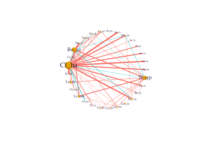

PLNmixture: model-based clustering

my_mixtures <- PLNmixture(Abundance ~ offset(log(Offset)), data = barents, clusters = 1:4,
                           control = PLNmixture_param(smoothing = "none"))

 Initialization...

 Adjusting 4 PLN mixture models.
    number of cluster = 1 
    number of cluster = 2 
    number of cluster = 3 
    number of cluster = 4 
 Post-treatments
 DONE!

myMixture <- getBestModel(my_mixtures)
plot(myMixture, "pca", main = "Clustering membership in the individual factor map")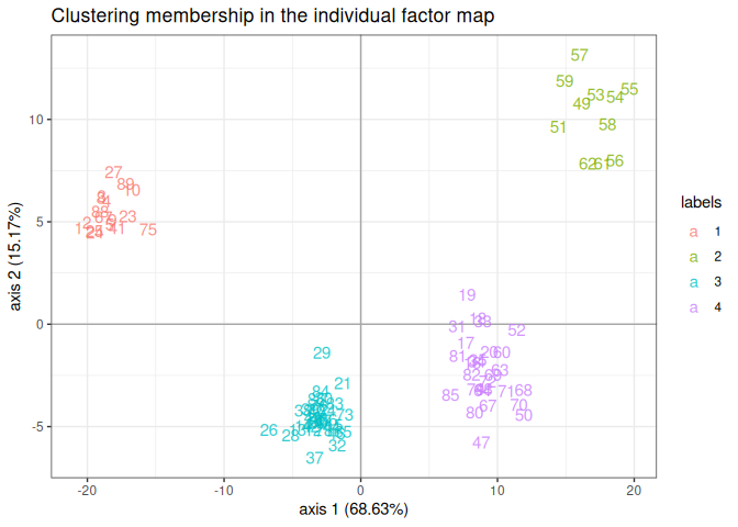

table(cluster = myMixture$memberships, zone = barents$zone)

       zone
cluster North South
      1     1    17
      2    11     0
      3    11    22
      4    21     6

PLNmodels: Poisson lognormal models for multivariate count data