Sparse structure estimation for multivariate count data with PLN-network

PLN team

2026-06-19

Preliminaries

This vignette illustrates the standard use of the PLNnetwork function and the methods accompanying the R6 Classes PLNnetworkfamily and PLNnetworkfit.

Requirements

The packages required for the analysis are PLNmodels plus some others for data manipulation and representation:

library(PLNmodels)
library(ggplot2)

Data set

We illustrate our point with the trichoptera data set, a full description of which can be found in the corresponding vignette. Data preparation is also detailed in the specific vignette.

data(trichoptera)
trichoptera <- prepare_data(trichoptera$Abundance, trichoptera$Covariate)

The trichoptera data frame stores a matrix of counts (trichoptera$Abundance), a matrix of offsets (trichoptera$Offset) and some vectors of covariates (trichoptera$Wind, trichoptera$Temperature, etc.)

Mathematical background

The network model for multivariate count data that we introduce in Chiquet et al. (2019) is a variant of the Poisson Lognormal model of Aitchison and Ho (1989), see the PLN vignette as a reminder. Compare to the standard PLN model we add a sparsity constraint on the inverse covariance matrix ${\boldsymbol\Sigma}^{-1}\triangleq \boldsymbol\Omega$ by means of the $\ell_1$-norm, such that $\|\boldsymbol\Omega\|_1 < c$. PLN-network is the equivalent of the sparse multivariate Gaussian model (Banerjee et al. 2008) in the PLN framework. It relates some $p$-dimensional observation vectors $\mathbf{Y}_i$ to some $p$-dimensional vectors of Gaussian latent variables $\mathbf{Z}_i$ as follows $$\begin{equation} \begin{array}{rcl} \text{latent space } & \mathbf{Z}_i \sim \mathcal{N}\left({\boldsymbol\mu},\boldsymbol\Omega^{-1}\right) & \|\boldsymbol\Omega\|_1 < c \\ \text{observation space } & Y_{ij} | Z_{ij} \quad \text{indep.} & Y_{ij} | Z_{ij} \sim \mathcal{P}\left(\exp\{Z_{ij}\}\right) \end{array} \end{equation}$$

The parameter ${\boldsymbol\mu}$ corresponds to the main effects and the latent covariance matrix $\boldsymbol\Sigma$ describes the underlying structure of dependence between the $p$ variables.

The $\ell_1$-penalty on $\boldsymbol\Omega$ induces sparsity and selection of important direct relationships between entities. Hence, the support of $\boldsymbol\Omega$ correspond to a network of underlying interactions. The sparsity level ($c$ in the above mathematical model), which corresponds to the number of edges in the network, is controlled by a penalty parameter in the optimization process sometimes referred to as $\lambda$. All mathematical details can be found in Chiquet et al. (2019).

Covariates and offsets

Just like PLN, PLN-network generalizes to a formulation close to a multivariate generalized linear model where the main effect is due to a linear combination of $d$ covariates $\mathbf{x}_i$ and to a vector $\mathbf{o}_i$ of $p$ offsets in sample $i$. The latent layer then reads $$\begin{equation} \mathbf{Z}_i \sim \mathcal{N}\left({\mathbf{o}_i + \mathbf{x}_i^\top\mathbf{B}},\boldsymbol\Omega^{-1}\right), \qquad \|\boldsymbol\Omega\|_1 < c , \end{equation}$$ where $\mathbf{B}$ is a $d\times p$ matrix of regression parameters.

Alternating optimization

Regularization via sparsification of $\boldsymbol\Omega$ and visualization of the consecutive network is the main objective in PLN-network. To reach this goal, we need to first estimate the model parameters. Inference in PLN-network focuses on the regression parameters $\mathbf{B}$ and the inverse covariance $\boldsymbol\Omega$. Technically speaking, we adopt a variational strategy to approximate the $\ell_1$-penalized log-likelihood function and optimize the consecutive sparse variational surrogate with an optimization scheme that alternates between two step

1. a gradient-ascent-step, performed with the CCSA algorithm of Svanberg (2002) implemented in the C++ library (Johnson 2011), which we link to the package.
2. a penalized log-likelihood step, performed with the graphical-Lasso of Friedman et al. (2008), implemented in the package fastglasso (Sustik and Calderhead 2012).

More technical details can be found in Chiquet et al. (2019)

Analysis of trichoptera data with a PLNnetwork model

In the package, the sparse PLN-network model is adjusted with the function PLNnetwork, which we review in this section. This function adjusts the model for a series of value of the penalty parameter controlling the number of edges in the network. It then provides a collection of objects with class PLNnetworkfit, corresponding to networks with different levels of density, all stored in an object with class PLNnetworkfamily.

Adjusting a collection of network - a.k.a. a regularization path

PLNnetwork finds an hopefully appropriate set of penalties on its own. This set can be controlled by the user, but use it with care and check details in ?PLNnetwork. The collection of models is fitted as follows:

network_models <- PLNnetwork(Abundance ~ 1 + offset(log(Offset)), data = trichoptera)

## 
##  Initialization...
##  Adjusting 30 PLN with sparse inverse covariance estimation
##  Joint optimization alternating gradient descent and graphical-lasso
##  sparsifying penalty = 2.123258  sparsifying penalty = 1.961192  sparsifying penalty = 1.811496  sparsifying penalty = 1.673226  sparsifying penalty = 1.54551   sparsifying penalty = 1.427542  sparsifying penalty = 1.318579  sparsifying penalty = 1.217933  sparsifying penalty = 1.124969  sparsifying penalty = 1.039101  sparsifying penalty = 0.9597877     sparsifying penalty = 0.886528  sparsifying penalty = 0.81886   sparsifying penalty = 0.7563572     sparsifying penalty = 0.6986251     sparsifying penalty = 0.6452996     sparsifying penalty = 0.5960444     sparsifying penalty = 0.5505489     sparsifying penalty = 0.508526  sparsifying penalty = 0.4697106     sparsifying penalty = 0.433858  sparsifying penalty = 0.400742  sparsifying penalty = 0.3701537     sparsifying penalty = 0.3419002     sparsifying penalty = 0.3158032     sparsifying penalty = 0.2916982     sparsifying penalty = 0.2694332     sparsifying penalty = 0.2488676     sparsifying penalty = 0.2298717     sparsifying penalty = 0.2123258 
##  Post-treatments
##  DONE!

Note the use of the formula object to specify the model, similar to the one used in the function PLN.

Structure of PLNnetworkfamily

The network_models variable is an R6 object with class PLNnetworkfamily, which comes with a couple of methods. The most basic is the show/print method, which sends a very basic summary of the estimation process:

network_models

## --------------------------------------------------------
## COLLECTION OF 30 POISSON LOGNORMAL MODELS
## --------------------------------------------------------
##  Task: Network Inference 
## ========================================================
##  - 30 penalties considered: from 0.2123258 to 2.123258 
##  - Best model (greater BIC): lambda = 0.47 
##  - Best model (greater EBIC): lambda = 0.756

One can also easily access the successive values of the criteria in the collection

network_models$criteria %>% head() %>% knitr::kable()

param	nb_param	loglik	BIC	AIC	ICL	n_edges	EBIC	pen_loglik	density	stability
2.123258	35	-1240.599	-1308.706	-1275.599	-2719.514	1	-1311.162	-1245.892	0.0069204	NA
1.961192	35	-1233.931	-1302.038	-1268.931	-2704.993	1	-1304.494	-1239.082	0.0069204	NA
1.811495	35	-1227.261	-1295.368	-1262.261	-2689.054	1	-1297.824	-1232.280	0.0069204	NA
1.673226	35	-1220.836	-1288.943	-1255.836	-2673.301	1	-1291.399	-1225.724	0.0069204	NA
1.545510	35	-1214.663	-1282.770	-1249.663	-2657.834	1	-1285.227	-1219.420	0.0069204	NA
1.427542	35	-1208.743	-1276.850	-1243.743	-2642.672	1	-1279.306	-1213.368	0.0069204	NA

A diagnostic of the optimization process is available via the convergence field:

network_models$convergence %>% head() %>% knitr::kable()

	param	nb_param	status	backend	objective	iterations	convergence
out	2.123258	35	3	newton	1240.599	20	2.382757e-05
elt	1.961192	35	3	newton	1233.931	15	8.428628e-06
elt.1	1.811495	35	3	newton	1227.261	16	9.377476e-06
elt.2	1.673226	35	3	newton	1220.836	16	9.633539e-06
elt.3	1.545510	35	3	newton	1214.663	16	9.636082e-06
elt.4	1.427542	35	3	newton	1208.743	16	9.5936e-06

An nicer view of this output comes with the option “diagnostic” in the plot method:

plot(network_models, "diagnostic")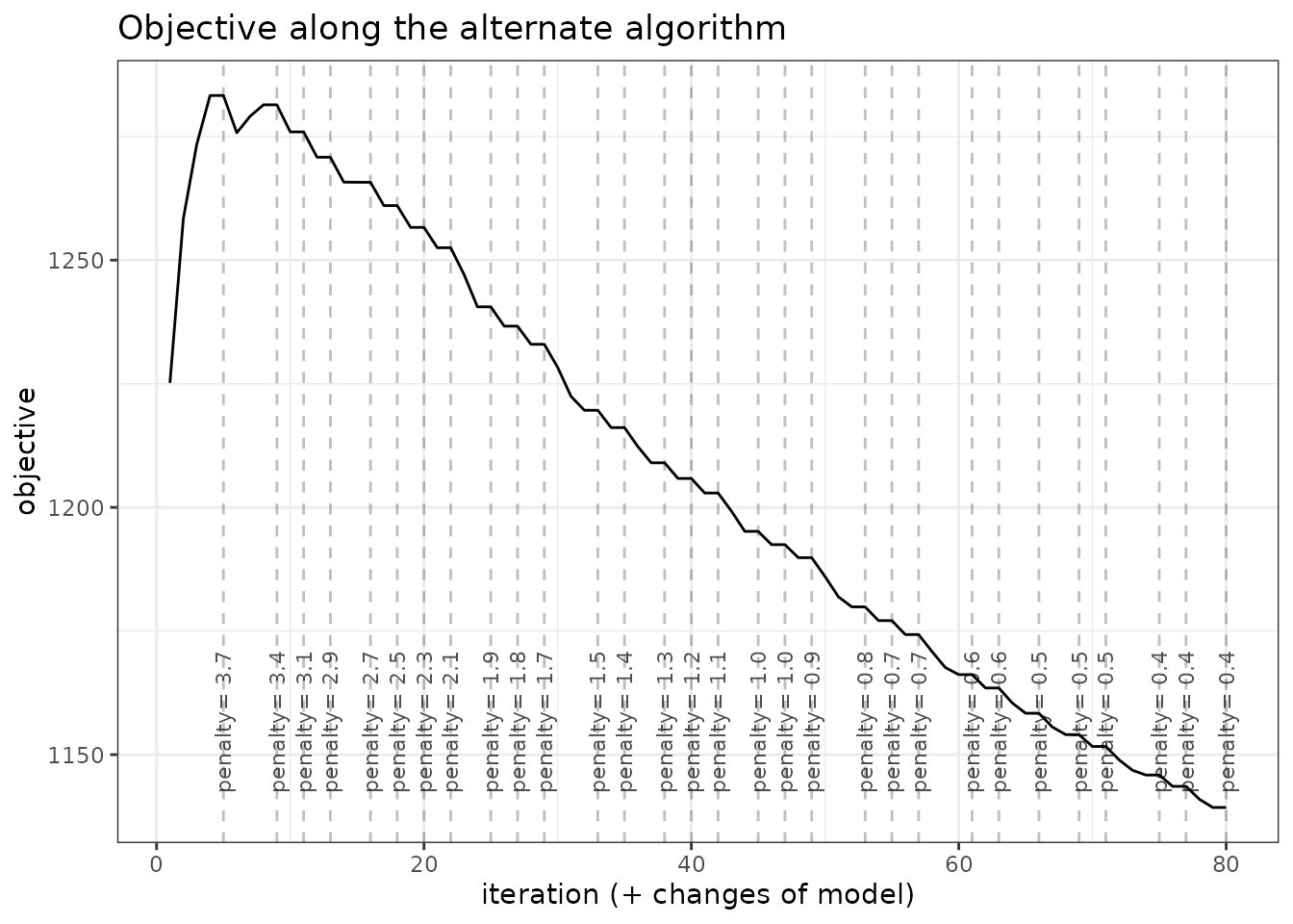

Exploring the path of networks

By default, the plot method of PLNnetworkfamily displays evolution of the criteria mentioned above, and is a good starting point for model selection:

plot(network_models)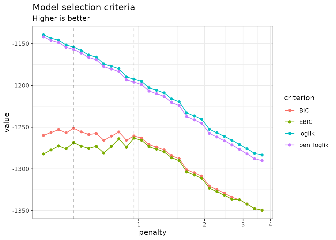

Note that we use the original definition of the BIC/ICL criterion ($\texttt{loglik} - \frac{1}{2}\texttt{pen}$), which is on the same scale as the log-likelihood. A popular alternative consists in using $-2\texttt{loglik} + \texttt{pen}$ instead. You can do so by specifying reverse = TRUE:

plot(network_models, reverse = TRUE)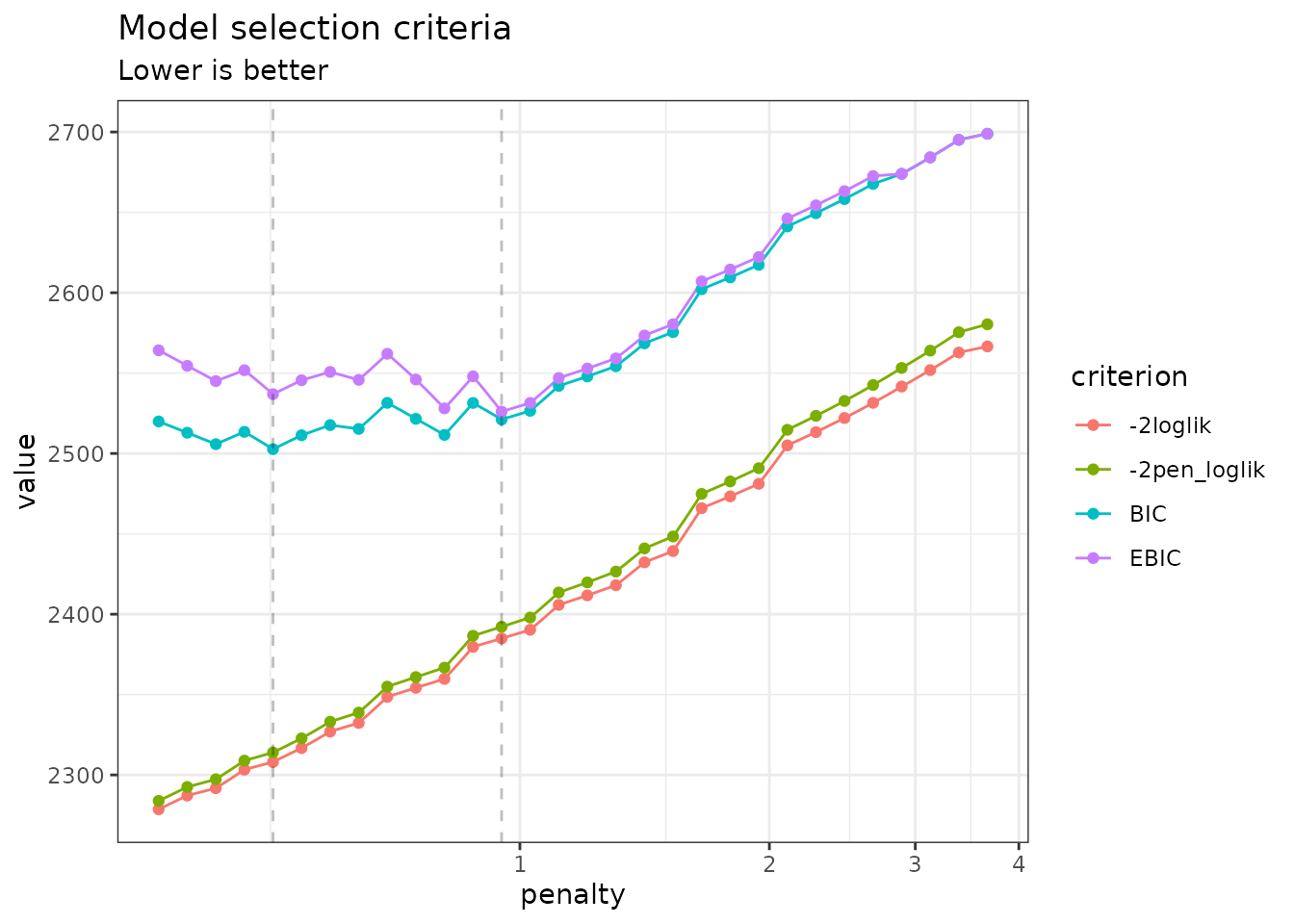

In this case, the variational lower bound of the log-likelihood is hopefully strictly increasing (or rather decreasing if using reverse = TRUE) with a lower level of penalty (meaning more edges in the network). The same holds true for the penalized counterpart of the variational surrogate. Generally, smoothness of these criteria is a good sanity check of optimization process. BIC and its extended-version high-dimensional version EBIC are classically used for selecting the correct amount of penalization with sparse estimator like the one used by PLN-network. However, we will consider later a more robust albeit more computationally intensive strategy to chose the appropriate number of edges in the network.

To pursue the analysis, we can represent the coefficient path (i.e., value of the edges in the network according to the penalty level) to see if some edges clearly come off. An alternative and more intuitive view consists in plotting the values of the partial correlations along the path, which can be obtained with the options corr = TRUE. To this end, we provide the S3 function coefficient_path:

coefficient_path(network_models, corr = TRUE) %>%
  ggplot(aes(x = Penalty, y = Coeff, group = Edge, colour = Edge)) +
    geom_line(show.legend = FALSE) +  coord_transform(x="log10") + theme_bw()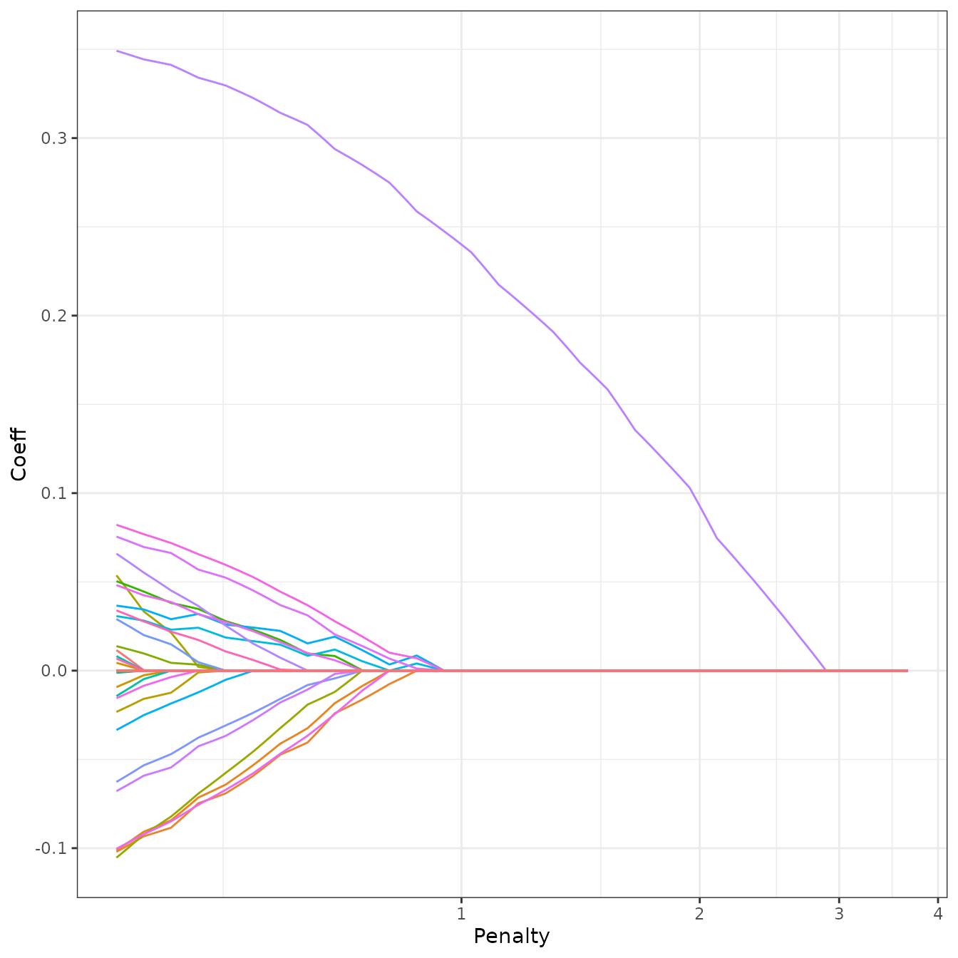

Model selection issue: choosing a network

To select a network with a specific level of penalty, one uses the getModel(lambda) S3 method. We can also extract the best model according to the BIC or EBIC with the method getBestModel().

model_pen <- getModel(network_models, network_models$penalties[20]) # give some sparsity
model_BIC <- getBestModel(network_models, "BIC")   # if no criteria is specified, the best BIC is used

An alternative strategy is to use StARS (Liu et al. 2010), which performs resampling to evaluate the robustness of the network along the path of solutions in a similar fashion as the stability selection approach of Meinshausen and Bühlmann (2010), but in a network inference context.

Resampling can be computationally demanding but is easily parallelized: the function stability_selection relies on parallel::mclapply to perform parallel computing. Set the number of workers with the mc.cores option (forking-based, so only effective on Unix-like systems; ignored on Windows):

options(mc.cores = 2)

We first invoke stability_selection explicitly for pedagogical purpose. In this case, we need to build our sub-samples manually:

n <- nrow(trichoptera)
subs <- replicate(10, sample.int(n, size = n/2), simplify = FALSE)
stability_selection(network_models, subsamples = subs)

## 
## Stability Selection for PLNnetwork: 
## subsampling: ++++++++++

Requesting ‘StARS’ in gestBestmodel automatically invokes stability_selection with 20 sub-samples, if it has not yet been run.

model_StARS <- getBestModel(network_models, "StARS")

When “StARS” is requested for the first time, getBestModel automatically calls the method stability_selection with the default parameters. After the first call, the stability path is available from the plot function:

plot(network_models, "stability")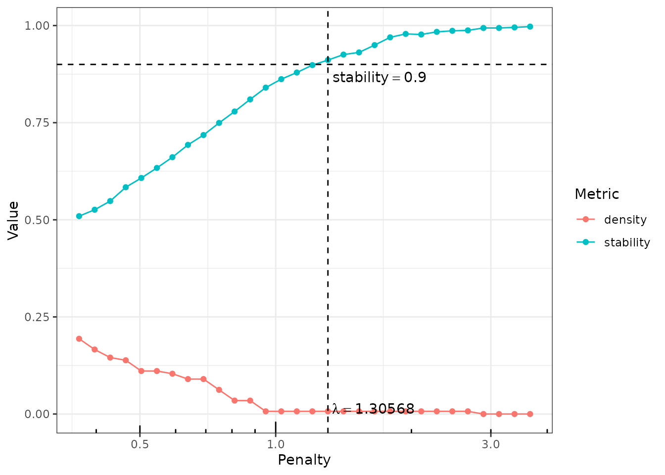

When you are done, do not forget to get back to the default (sequential) behavior.

options(mc.cores = 1)

Structure of a PLNnetworkfit

The variables model_BIC, model_StARS and model_pen are other R6Class objects with class PLNnetworkfit. They all inherits from the class PLNfit and thus own all its methods, with a couple of specific one, mostly for network visualization purposes. Most fields and methods are recalled when such an object is printed:

model_StARS

## Poisson Lognormal with sparse inverse covariance (penalty = 1.04)
## ==================================================================
##  nb_param   loglik       BIC      AIC       ICL n_edges      EBIC pen_loglik
##        35 -1187.49 -1255.597 -1222.49 -2585.114       1 -1258.053  -1191.596
##  density
##    0.007
## ==================================================================
## * Useful fields
##     $model_par, $latent, $latent_pos, $var_par, $optim_par
##     $loglik, $BIC, $ICL, $loglik_vec, $nb_param, $criteria
## * Useful S3 methods
##     print(), coef(), sigma(), vcov(), fitted()
##     predict(), predict_cond(), standard_error()
## * Additional fields for sparse network
##     $EBIC, $density, $penalty 
## * Additional S3 methods for network
##     plot.PLNnetworkfit()

The plot method provides a quick representation of the inferred network, with various options (either as a matrix, a graph, and always send back the plotted object invisibly if users needs to perform additional analyses).

my_graph <- plot(model_StARS, plot = FALSE)
my_graph

## IGRAPH a1a64ea UNW- 17 1 -- 
## + attr: name (v/c), label (v/c), label.cex (v/n), size (v/n),
## | label.color (v/c), weight (e/n), color (e/c), width (e/n)
## + edge from a1a64ea (vertex names):
## [1] Hfo--Hsp

plot(model_StARS)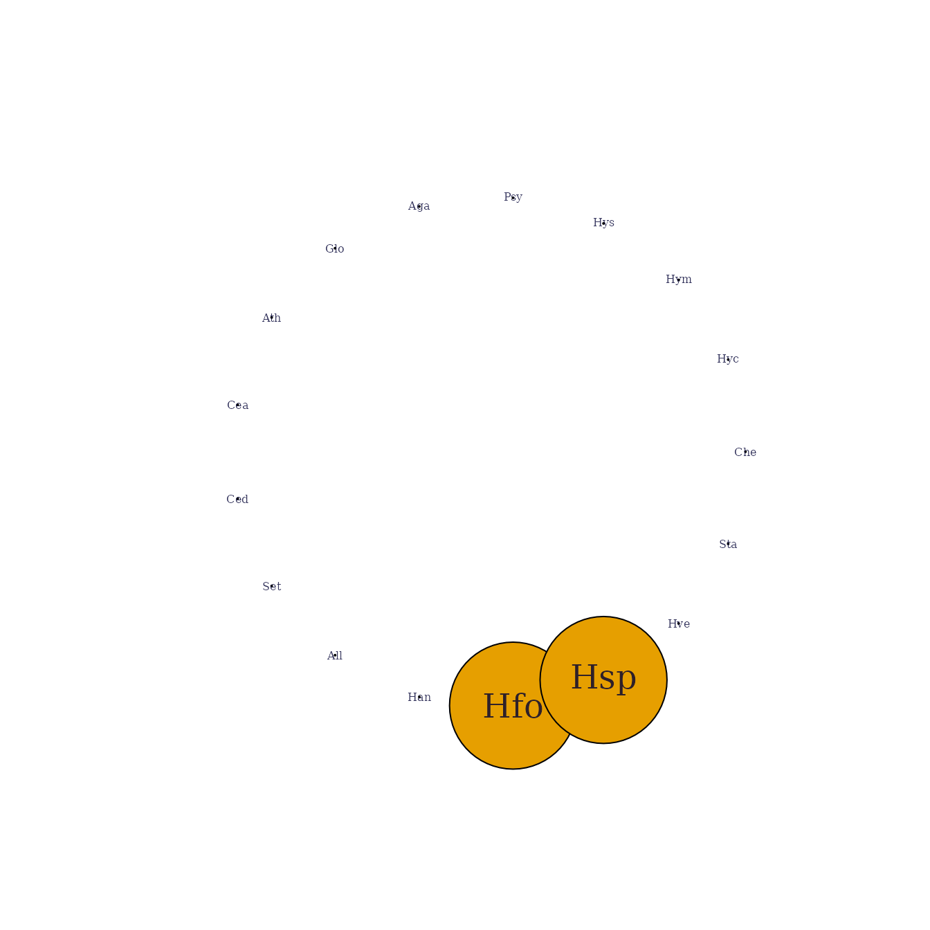

plot(model_StARS, type = "support", output = "corrplot")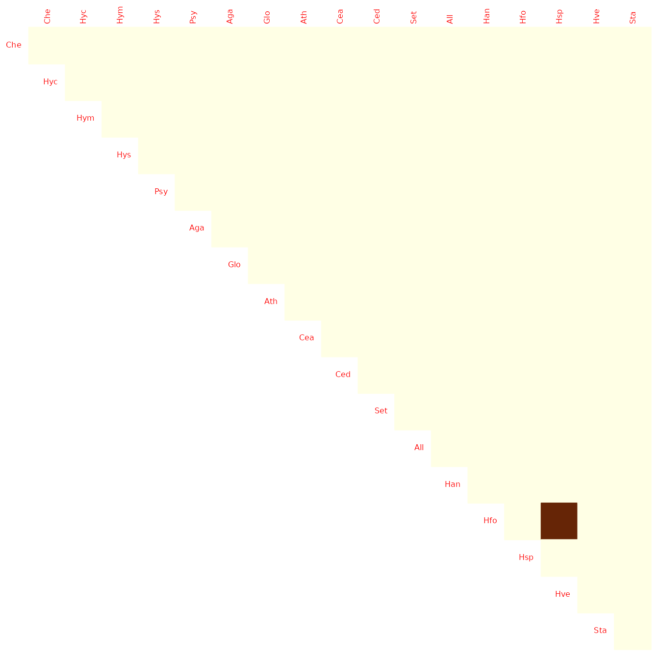

We can finally check that the fitted value of the counts – even with sparse regularization of the covariance matrix – are close to the observed ones:

data.frame(
  fitted   = as.vector(fitted(model_StARS)),
  observed = as.vector(trichoptera$Abundance)
) %>%
  ggplot(aes(x = observed, y = fitted)) +
    geom_point(size = .5, alpha =.25 ) +
    scale_x_log10(limits = c(1,1000)) +
    scale_y_log10(limits = c(1,1000)) +
    theme_bw() + annotation_logticks()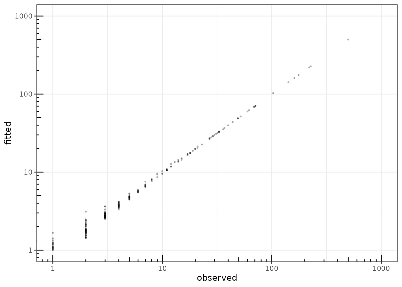

fitted value vs. observation

References

Aitchison, J., and C. H. Ho. 1989. “The Multivariate Poisson-Log Normal Distribution.” Biometrika 76 (4): 643–53.

Banerjee, Onureena, Laurent El Ghaoui, and Alexandre d’Aspremont. 2008. “Model Selection Through Sparse Maximum Likelihood Estimation for Multivariate Gaussian or Binary Data.” Journal of Machine Learning Research 9 (Mar): 485–516.

Chiquet, Julien, Stephane Robin, and Mahendra Mariadassou. 2019. “Variational Inference for Sparse Network Reconstruction from Count Data.” In Proceedings of the 36th International Conference on Machine Learning, edited by Kamalika Chaudhuri and Ruslan Salakhutdinov, vol. 97. Proceedings of Machine Learning Research. PMLR. http://proceedings.mlr.press/v97/chiquet19a.html.

Friedman, J., T. Hastie, and R. Tibshirani. 2008. “Sparse Inverse Covariance Estimation with the Graphical Lasso.” Biostatistics 9 (3): 432–41.

Johnson, Steven G. 2011. The NLopt Nonlinear-Optimization Package. https://nlopt.readthedocs.io/en/latest/.

Liu, Han, Kathryn Roeder, and Larry Wasserman. 2010. “Stability Approach to Regularization Selection (StARS) for High Dimensional Graphical Models.” Proceedings of the 23rd International Conference on Neural Information Processing Systems - Volume 2 (USA), 1432–40.

Meinshausen, Nicolai, and Peter Bühlmann. 2010. “Stability Selection.” Journal of the Royal Statistical Society: Series B (Statistical Methodology) 72 (4): 417–73.

Sustik, Mátyás A, and Ben Calderhead. 2012. “GLASSOFAST: An Efficient GLASSO Implementation.” UTCS Technical Report TR-12-29 2012.

Svanberg, Krister. 2002. “A Class of Globally Convergent Optimization Methods Based on Conservative Convex Separable Approximations.” SIAM Journal on Optimization 12 (2): 555–73.